10  gLV 模型

GLV 模型的数学表达为：

\[ \dfrac{d x_i(t)}{d t} = x_i(t) \left(a_i + \sum_{j} B_{ij} x_j(t) \right) \]

可以被缩写为

\[ \dfrac{d x}{d t} = D(x) (a + B x) \]

或者

\[ \dfrac{dx(t)}{dt} = D(x(t))(r + A x(t)) \]

where \(x(t)\) is a (column) vector of length \(n\) containing the densities of all populations \(1, \ldots, n\) at time \(t\), \(r\) is a vector of “intrinsic growth rates” (or death rates, when negative), measuring the growth (decline) of population \(i\) when grown alone at low density, and \(A\) is a \(n \times n\) matrix of interaction coefficients. We use \(D(x)\) to denote the diagonal matrix with \(x\) on the diagonal.

其中， \(x(t)\) 是长度为 的（列）向量，表示 \(1, \ldots, n\) 物种在 \(t\) 时的种群密度；\(r\) 是这些物种的内禀增长率（若为负值则相当于死亡率），表示物种 \(i\) 在单独生长、种群数量低的时候种群数量的增长（或减少）情况；\(A\) 是一个 \(n \times n\) 的种间相互作用矩阵。\(D(x)\) 用来表示对角元素为 \(x\) 的对角矩阵。

10.1 单物种群体

The simplest case to study is that of a single population, in which case the equation becomes that of the logistic growth:

\[ \dfrac{dx(t)}{dt} = x(t)(r + a x(t)) \]

This is a separable ODE, with solution:

\[ x(t) = \frac{r}{e^{-r \left(k+t\right)}-a} \]

where \(k\) is a constant. Setting \(x(0) = x_0\) (i.e., providing an initial condition), solving for the constant and substituting, we obtain:

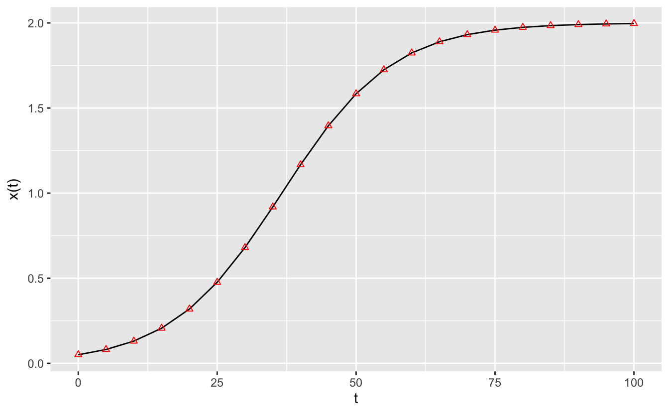
\[ x(t) = \frac{r {x_0} e^{r t}}{r-a {x_0} \left(e^{r t}-1\right)} \] As such, provided with the parameters \(r\) and \(a\), as well as an initial condition, we can determine the population size for any time \(t\). For example, in R:

pacman::p_load("deSolve") # integrate ODEs
pacman::p_load("tidyverse") # plotting and wrangling
# define the differential equation
logistic_growth <- function(t, x, parameters){
  with(as.list(c(x, parameters)), {
    dxdt <- x * (r + a * x)
    list(dxdt)
  })
}
# define parameters, integration time, initial conditions
times <- seq(0, 100, by = 5)
x0 <- 0.05
r <- 0.1
a <- -0.05
parameters <- list(r = r, a = a)
# solve numerically
out <- ode(y = x0, times = times, 
           func = logistic_growth, parms = parameters, 
           method = "ode45")
# now compute analytically
solution <- r * x0 * exp(r * times) / (r - a * x0 * (exp(r * times) - 1))
# use ggplot to plot
res <- tibble(time = out[,1], x_t = out[,2], x_sol = solution)
ggplot(data = res) + aes(x = time, y = x_t) + 
  geom_line() + 
  geom_point(aes(x = time, y = x_sol), colour = "red", shape = 2) + 
  ylab(expression("x(t)")) + xlab(expression("t"))

If \(a < 0\) and \(r > 0\), the population started at any positive value eventually reaches an equilibrium, which we can find by setting \(dx(t)/dt = 0\) and considering \(x \neq 0\):

\[ (r + a x) = 0 \to x = -\frac{r}{a} \]